Dale Barr (@datacmdr) recently had a nice blog post about coding categorical predictors, which reminded me to share my thoughts about multiple pairwise comparisons for categorical predictors in growth curve analysis. As Dale pointed out in his post, the R default is to treat the reference level of a factor as a baseline and to estimate parameters for each of the remaining levels. This will give pairwise comparisons for each of the other levels with the baseline, but not among those other levels. Here's a simple example using the
Here are the data:
Now let's fit the model:
The Intercept parameter (31.5) is the weight of the "Diet 1" chicks at birth, and the Time parameter (6.7) is their (linear) rate of growth. The Diet2, Diet3, and Diet4 parameters are the birth weights for the chicks in those diet groups relative to Diet 1; the Time:Diet2, Time:Diet3, and Time:Diet4 parameters are the relative slopes -- these are the ones that capture the different effects of diet on rate of growth. But that's rate of growth relative to Diet 1, what if we want to check for differences between Diet 2 and Diet 3?
One option is to re-level the factor so that Diet 2 becomes the reference and the parameters are estimated relative to that:
That worked fine, though it would be kind of annoying and repetitive to have to cycle through all different re-levelings. Especially since we actually have all of the relevant information in the original parameter estimates, we just need to compare them directly to one another. For example, in the original model, the parameter estimates for the growth rate for Diet 2 (Time:Diet2) was 1.896 and for Diet 3 (Time:Diet3) it was 4.71. If we take the difference between those, we get 2.814, which is exactly the parameter estimate for Diet 3 relative to Diet 2 in the releveled model (Time:DietReleveled3). The
First, we need to set up a contrast matrix that defines the comparisons that we want to test. Each column in this matrix corresponds to a parameter estimate from the original model, in the order that they appear in the output. So the first column corresponds to "(Intercept)", the second column to "Time", the sixth column to "Time:Diet2", etc. Each row in the contrast matrix corresponds to a contrast that you want to test and the elements in the matrix are weights for that contrast. The simplest case is when the contrast you want to test corresponds to an estimated parameter: you put a 1 in that column and a 0 in all of the others. For example, to test "Time:Diet1 vs. Time:Diet2" you just put a 1 in the sixth column for the Time:Diet2 parameter. If you want to compare two estimated parameters to one another, you put a -1 in one of their columns and a 1 in the other. Here's the contrast matrix for testing all pairwise slope differences:
Now we can use this contrast matrix to test the pairwise comparisons using the
This gives us the parameter estimates, standard errors, z-values for each of those comparisons, and adjusted p-values (i.e., corrected for multiple comparisons). If you don't like the default correction, you can change it or suppress it altogether by doing this:
Thanks to Scott Jackson for helping me figure out how to use the contrast matrix.
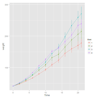
ChickWeight data set (part of the datasets package). As a reminder, this data set is from an experiment on the effect of diet on early growth of chicks. There were 50 chicks, each fed one of 4 diets, and their weights were measured up to 12 times over the first 3 weeks after they were born.Here are the data:
ggplot(ChickWeight, aes(Time, weight, color = Diet))
 + stat_summary(fun.y = mean, geom = "line")
 + stat_summary(fun.data = mean_se, geom = "pointrange")

Now let's fit the model:
m <- lmer(weight ~ Time * Diet + (1 | Chick),
    data = ChickWeight, REML = F)
print(m, corr = F)
## Linear mixed model fit by maximum likelihood
## Formula: weight ~ Time * Diet + (1 | Chick)
##    Data: ChickWeight
##   AIC  BIC logLik deviance REMLdev
##  5508 5552  -2744     5488    5467
## Random effects:
##  Groups   Name        Variance Std.Dev.
##  Chick    (Intercept) 498      22.3
##  Residual             638      25.3
## Number of obs: 578, groups: Chick, 50
##
## Fixed effects:
##             Estimate Std. Error t value
## (Intercept)   31.508      5.911    5.33
## Time           6.713      0.257   26.09
## Diet2         -2.874     10.191   -0.28
## Diet3        -13.258     10.191   -1.30
## Diet4         -0.398     10.200   -0.04
## Time:Diet2     1.896      0.427    4.44
## Time:Diet3     4.710      0.427   11.04
## Time:Diet4     2.949      0.432    6.82
One option is to re-level the factor so that Diet 2 becomes the reference and the parameters are estimated relative to that:
ChickWeight$DietReleveled <- relevel(ChickWeight$Diet, "2")
m.2 <- lmer(weight ~ Time * DietReleveled + (1 | Chick),
    data = ChickWeight, REML = F)
print(m.2, corr = F)
## Linear mixed model fit by maximum likelihood
## Formula: weight ~ Time * DietReleveled + (1 | Chick)
##    Data: ChickWeight
##   AIC  BIC logLik deviance REMLdev
##  5508 5552  -2744     5488    5467
## Random effects:
##  Groups   Name        Variance Std.Dev.
##  Chick    (Intercept) 498      22.3
##  Residual             638      25.3
## Number of obs: 578, groups: Chick, 50
##
## Fixed effects:
##                     Estimate Std. Error t value
## (Intercept)           28.634      8.302    3.45
## Time                   8.609      0.340   25.29
## DietReleveled1         2.874     10.191    0.28
## DietReleveled3       -10.383     11.740   -0.88
## DietReleveled4         2.476     11.748    0.21
## Time:DietReleveled1   -1.896      0.427   -4.44
## Time:DietReleveled3    2.814      0.481    5.84
## Time:DietReleveled4    1.053      0.486    2.17
multcomp package provides a way to do this sort of comparison using just the original model.First, we need to set up a contrast matrix that defines the comparisons that we want to test. Each column in this matrix corresponds to a parameter estimate from the original model, in the order that they appear in the output. So the first column corresponds to "(Intercept)", the second column to "Time", the sixth column to "Time:Diet2", etc. Each row in the contrast matrix corresponds to a contrast that you want to test and the elements in the matrix are weights for that contrast. The simplest case is when the contrast you want to test corresponds to an estimated parameter: you put a 1 in that column and a 0 in all of the others. For example, to test "Time:Diet1 vs. Time:Diet2" you just put a 1 in the sixth column for the Time:Diet2 parameter. If you want to compare two estimated parameters to one another, you put a -1 in one of their columns and a 1 in the other. Here's the contrast matrix for testing all pairwise slope differences:
contrast.matrix <- rbind(
    `Time:Diet1 vs. Time:Diet2` = c(0, 0, 0, 0, 0, 1, 0, 0),
    `Time:Diet1 vs. Time:Diet3` = c(0, 0, 0, 0, 0, 0, 1, 0),
    `Time:Diet1 vs. Time:Diet4` = c(0, 0, 0, 0, 0, 0, 0, 1),
    `Time:Diet2 vs. Time:Diet3` = c(0, 0, 0, 0, 0, -1, 1, 0),
    `Time:Diet2 vs. Time:Diet4` = c(0, 0, 0, 0, 0, -1, 0, 1),
    `Time:Diet3 vs. Time:Diet4` = c(0, 0, 0, 0, 0, 0, -1, 1))
glht function from the multcomp package:library(multcomp) comps <- glht(m, contrast.matrix) summary(comps)
##
##   Simultaneous Tests for General Linear Hypotheses
##
## Fit: lmer(formula = weight ~ Time * Diet + (1 | Chick),
##     data = ChickWeight, REML = F)
##
## Linear Hypotheses:
##                                Estimate Std. Error z value Pr(>|z|)
## Time:Diet1 vs. Time:Diet2 == 0    1.896      0.427    4.44   <0 ---="" --="" -1.760="" -3.62="" .001="" 0.0016="" 0.001="" 0.01="" 0.05="" 0.1321="" 0.1="" 0.427="" 0.432="" 0.481="" 0.486="" 0="" 1.053="" 11.04="" 1="" 2.17="" 2.814="" 2.949="" 4.710="" 5.84="" 6.82="" codes:="" djusted="" method="" p="" pre="" reported="" signif.="" single-step="" time:diet1="" time:diet2="" time:diet3="" time:diet4="=" values="" vs.="">
summary(glht(m, contrast.matrix), test = adjusted("none"))
##
##   Simultaneous Tests for General Linear Hypotheses
##
## Fit: lmer(formula = weight ~ Time * Diet + (1 | Chick),
##     data = ChickWeight, REML = F)
##
## Linear Hypotheses:
##                                Estimate Std. Error z value Pr(>|z|)
## Time:Diet1 vs. Time:Diet2 == 0    1.896      0.427    4.44  8.9e-06 ***
## Time:Diet1 vs. Time:Diet3 == 0    4.710      0.427   11.04  < 2e-16 ***
## Time:Diet1 vs. Time:Diet4 == 0    2.949      0.432    6.82  8.9e-12 ***
## Time:Diet2 vs. Time:Diet3 == 0    2.814      0.481    5.84  5.1e-09 ***
## Time:Diet2 vs. Time:Diet4 == 0    1.053      0.486    2.17  0.03031 *
## Time:Diet3 vs. Time:Diet4 == 0   -1.760      0.486   -3.62  0.00029 ***
## ---
## Signif. codes:  0 '***' 0.001 '**' 0.01 '*' 0.05 '.' 0.1 ' ' 1
## (Adjusted p values reported -- none method)
Thank you for an interesting and informative post, Dan! If we wanted to test differences in specific diets at each time point, how would we set up our contrasts? In particular, would we need to specify Time as a factor (i.e., categorical variable) so that we can control which levels of time we are looking at when comparing diets?
ReplyDeleteIn general, I prefer to treat continuous predictors (like Time) as continuous and to evaluate effects of conditions (like Diet) on patterns/trajectories over those continuous predictors (intercepts, slopes, curvature parameters, etc.). Most of the phenomena I deal with evolve gradually over time, so my default is to be suspicious of claims that X occurred at time T; especially if it that claim is based on a p-value being less than <0.05 at T but not T-1. If the time points are discrete events (for example, pre-test, post-test, and follow-up), then it can make sense to treat Time as a factor and apply the contrast matrix logic to get pairwise comparisons at different (discrete) time points -- exactly as you suggest.
DeleteHi Dan, thanks for this helpful post. I'm trying to apply it to some of my own work, and I'm curious: if you wanted to do a 'contrast of contrasts,' would you just subtract one row in the contrast matrix from another?
DeleteFor example, say you wanted to know the difference between 'Time:Diet3 vs. Time:Diet4' and 'Time:Diet3 vs. Time:Diet4'. Would you subtract (0, 0, 0, 0, 0, 0, -1, 1) from (0, 0, 0, 0, 0, -1, 0, 1) and therefore get (0,0,0,0,1,-1,0)? You would then run the contrast c(0,0,0,1,-1,0) with the same model above ('m') to get this contrast of contrasts?
This is the approach I have been using, just wanted to confirm with someone else who had experience using this approach.
Thanks,
Noah Sokol (noah.sokol@yale.edu)
Hi Noah,
DeleteI'm not quite sure what you're after with the "contrast of contrasts". When you compare "T:D2 vs. T:D4" against "T:D3 vs. T:D4", T:D4 is in both and it cancels out, so you end up with a "T:D2 vs. T:D3" comparison. Your contrast matrix arithmetic was internally consistent, so it produced that exact vector, which was already in the matrix (except with opposite signs, but it's the same contrast). Hope that helps.
Thank you Dan for this amazing posting. It really helped me to understand how to make a contrast matrix. But, I am still wondering how to do that when there are more than two factors. For example, in this ChickWeight dataset, we may add one more column for gender (F for female and M for male). Then we will have 8 lines instead of 4 (F1 to F4, M1 to M4). In this case, do you happen to know to make a contrast matrix? I think I can make contrasts within one gender like
ReplyDeletetime:F1 vs. time:F2
time:F1 vs. time:F3
time:F1 vs. time:F4
time:F2 vs. time:F3
time:F2 vs. time:F4
time F3 vs. time:F4
But, if I want to compare the slopes across genders and diets like
time:F1 vs. time:M1
time:F1 vs. time:M2
.....
I have little idea on making contrasts. If you know some tips about this, I will really appreciate it!
Thank you,
KJ
Hi Dan,
ReplyDeleteThanks for this tutorial - super helpful! I had one follow-up question, do you know how this might change if there was a quadratic for time? The particular model I am fitting has linear and a quadratic terms for age (and then cohort as a a categorical predictor with 4 levels), so I wonder how this affects the contrast coding?
Thanks in advance for any help you may have to offer! =:-]
Hi Libby,
DeleteSorry it took me a long time to get to this, and I'm not sure my answer will be relevant any more, but here goes. The logic is the same, you just have to extend the structure of the contrast matrix to the quadratic Time^2 terms.
Hi Dan,
ReplyDeleteThanks for the tutorial.. Super helpful. I wonder if we could get confidence intervals for the comparisons too using glht. Thanks!
:)
glht returns parameter estimates for the comparisons along with SE for those estimates. You can use the SE to compute confidence intervals if you want. I also like the effects package for computing estimates and CI.
Delete